Retail Operating System
Save Hundreds of Hours. Eliminate Errors.
Multi-channel merchants and wholesalers turn to Brightpearl to streamline operations, boost efficiency and stay ahead in a fast-changing retail landscape.
Brightpearl customers are free to focus on growth. They use our Automation Engine to…
- Save two months a year, on average
- Reduce human errors by 65%
- Lower labor costs by 50%
5,000+ pioneering brands rely on Brightpearl to grow further and faster
Tough times don’t last.
Brightpearl customers do.
A global market slowdown. A supply chain crisis. Wavering consumer demand. Rising costs. It’s a tricky time to be in retail. But it doesn’t have to be.
Out of the chaos, opportunities are emerging. Be ready to seize them with Brightpearl.
Automate your operations, intelligently plan your inventory and make your investments go further with our #1 Retail Operating System.

Free up your time, keep up your profits
by automating (almost) everything
Right now, your business needs you to spend your time innovating, adapting and seizing opportunities – not getting bogged down by tedious, low-profit tasks.
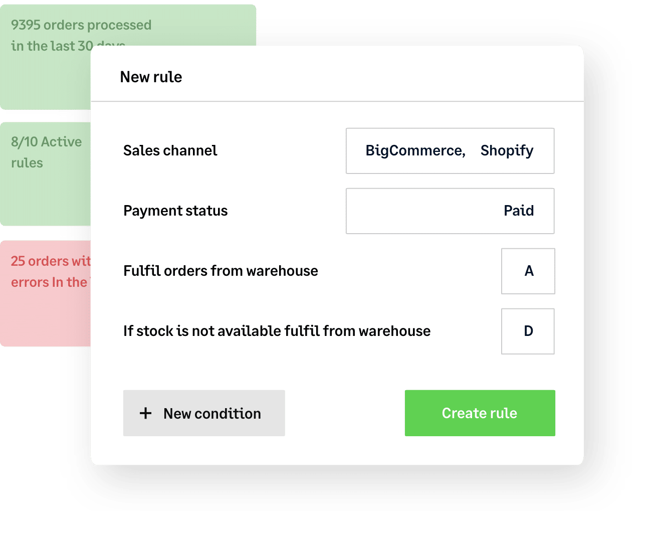
Easily automate everything from complex order fulfillment and multi-location inventory management to shipping and accounting with Brightpearl’s powerful Automation Engine. Save 1000s of hours and focus your energy where it counts.
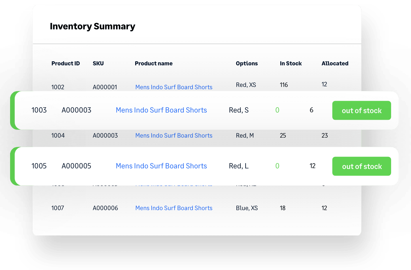
Dodge supply chain
curveballs
with smart sales forecasting and inventory planning
Delayed orders? Warehouse full of stock you can’t shift? Best-sellers always running low? You need an advanced inventory planning solution that can handle unpredictable demand and supply chain disruption to keep your cash flow healthy. You need Brightpearl.
Get buying recommendations based on accurate sales forecasting so you always know what to order, how much to order and when to order it. You can even factor in rapidly-changing trends and sudden market shifts into your planning – in the current market, it’s the only way to get ahead.
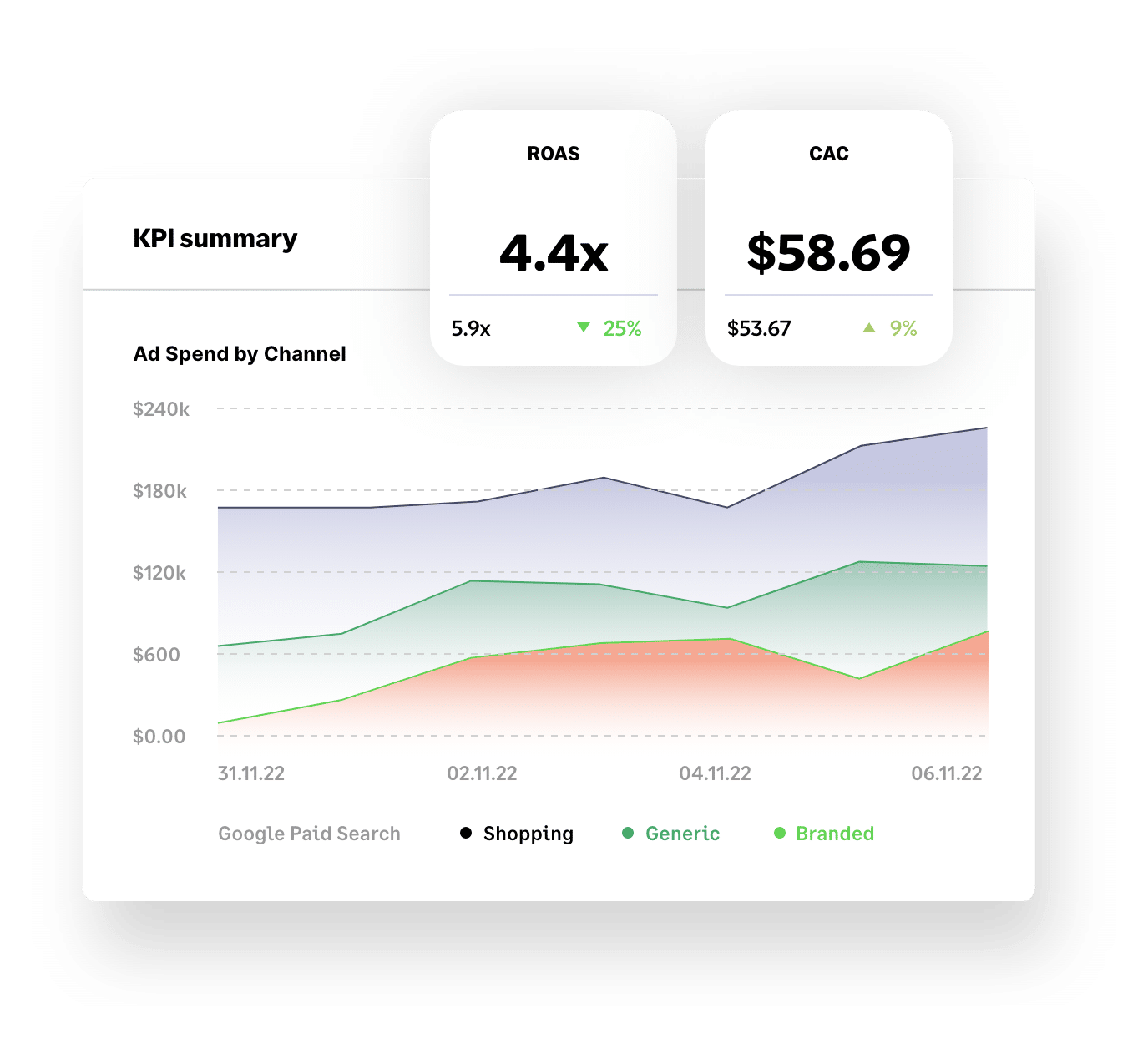
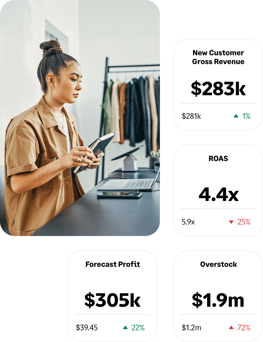
Get more bang
for your buck
with advanced insights + analysis
Make smarter decisions and grow your business faster with Brightpearl’s retail analytics.
Yes, our business intelligence tools include key KPIs like Customer Acquisition Cost (CAC), Lifetime Value (LTV), best-selling products and paid search and social performance – but, unlike other tools, our data is accurate and super easy to navigate.
You can even access industry benchmarks to see how your performance compares to your competition.
Be where your
customers are
with a huge range of Plug & Play apps
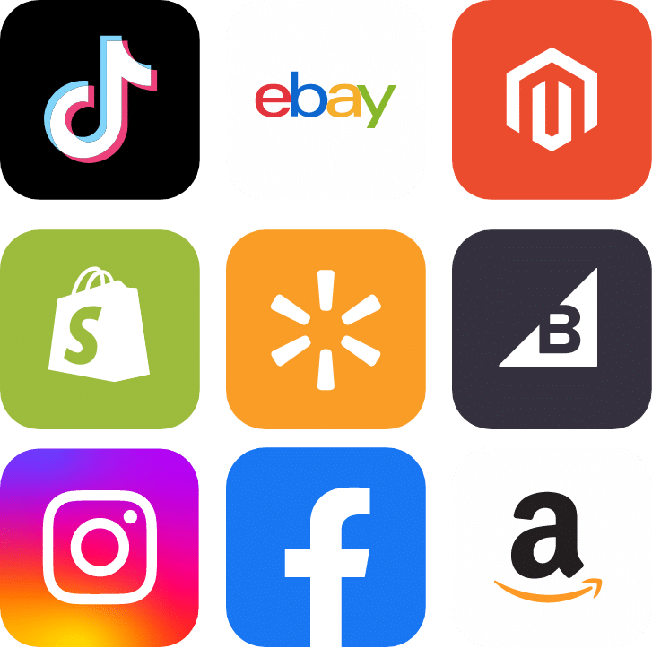
Attracting new customers (and being where your current ones hang out online) is key to growth but can introduce complexity. Brightpearl’s market-disrupting library of Plug & Play integrations makes it simple.
Add new sales channels – including TikTok, Instagram, live stream platforms and more – in minutes. Curate an ever-changing roster of the latest tech tools, as and when your business needs them. Access deep APIs and a certified network of development partners so that where other brands falter, you can soar.

Expert support
at every step
with our end-to-end services
The right software is important, but it’s not enough on its own. To unlock your unique growth potential, it has to be optimized by experts and backed up by training and support.
At Brightpearl, our retail experts are with you every step of the way. From flawless implementation with a proven 97% success rate and bespoke onboarding training to ongoing consulting and 24/7 support, we’ll ensure you get the very best from Brightpearl.

Our customers
Trusted by merchants
in every industry
Why Brightpearl
Cutting-edge software
Leading tech backed up with a 97% implementation success rate
Part of Sage Group Plc
We're built on a solid foundation, which helps us invest in product R&D
Certified Shopify Partner
We’re proud to be founding member of Shopify’s global ERP Program
Proven track record
We power millions of orders a month for some of the world’s biggest brands
Excellent reviews
We’ve earned great reviews from customers, including 4.5 stars on Trustpilot
Expert support
Our experts are always on hand for training and support
Brightpearl App Store
Instantly connect Brightpearl with the tools you need
to grow fearlessly
Shopify
E-Commerce
Amazon
E-Commerce
BigCommerce
E-Commerce
Magento
E-Commerce
eBay
E-Commerce
Quickbooks
Accounting
Lightspeed
E-Commerce
Shipstation
Shipping
Dotdigital
E-Commerce
Xero
Accounting
Square
E-Commerce
Klaviyo
E-Commerce
More reading
Events, News and Insights
Got questions
Ready to reach your potential? Book a demo today to see how Brightpearl can help you do business better.
Book a demo